Notes on ICML 2021 tutorial about Sparsity in Deep Learning
ㅤ
ICML 2021 Tutorial: Sparsity in Deep Learning: Pruning growth for efficient inference and training in neural networks
Gaoxiang: I came across this tutorial when volunteering in ICML 2021, and I found it’s very useful for people who’re new like me to understand Sparsity in Deep Learning today. This tutorial is given by Torsten Hoffler, Dan Alisarh, Tal Ben-nun, Nikoli Dryden, Alexandra Peste. For this tutorial, check their most recent paper Sparsity in Deep Learning: Pruning and growth for efficient inference and training in neural networks on arXiv.
Introduction and Overview
Why do we care about sparisity? Before we answer this question, let’s dig into how to compress and optimize models. For example, one can compress the model by using smaller dense models, represent matrixes by a factored decomposition, use low precision values, share the parameters across neurons, etc; however, one can also apply sparsity to achieve the same goal, which is the main focus on this blog.
The intuition of the sparity comes from that fact that not all features are always relevant. If we represent feature vectors in (sparse) vector space, then the model would be less overfitting becuase it has less parameters. It also helps in interpretability but not neccesarily in large models with lots of paramters. More importantly, it helps parsimony, which means we only store the essences that we need to store. For intance, you can read the following sentence the f_t_re wi_l b_ sp_rs_ even though it’s not complete. Even though it only has 30% of the letters but it’s still working for us, for the neural networks that are in our brains.
An example to relate to - CNNs from a spartisty viewpoint
To give you a example that you’re familiar with when working with neural networks, let’s look at the following images.
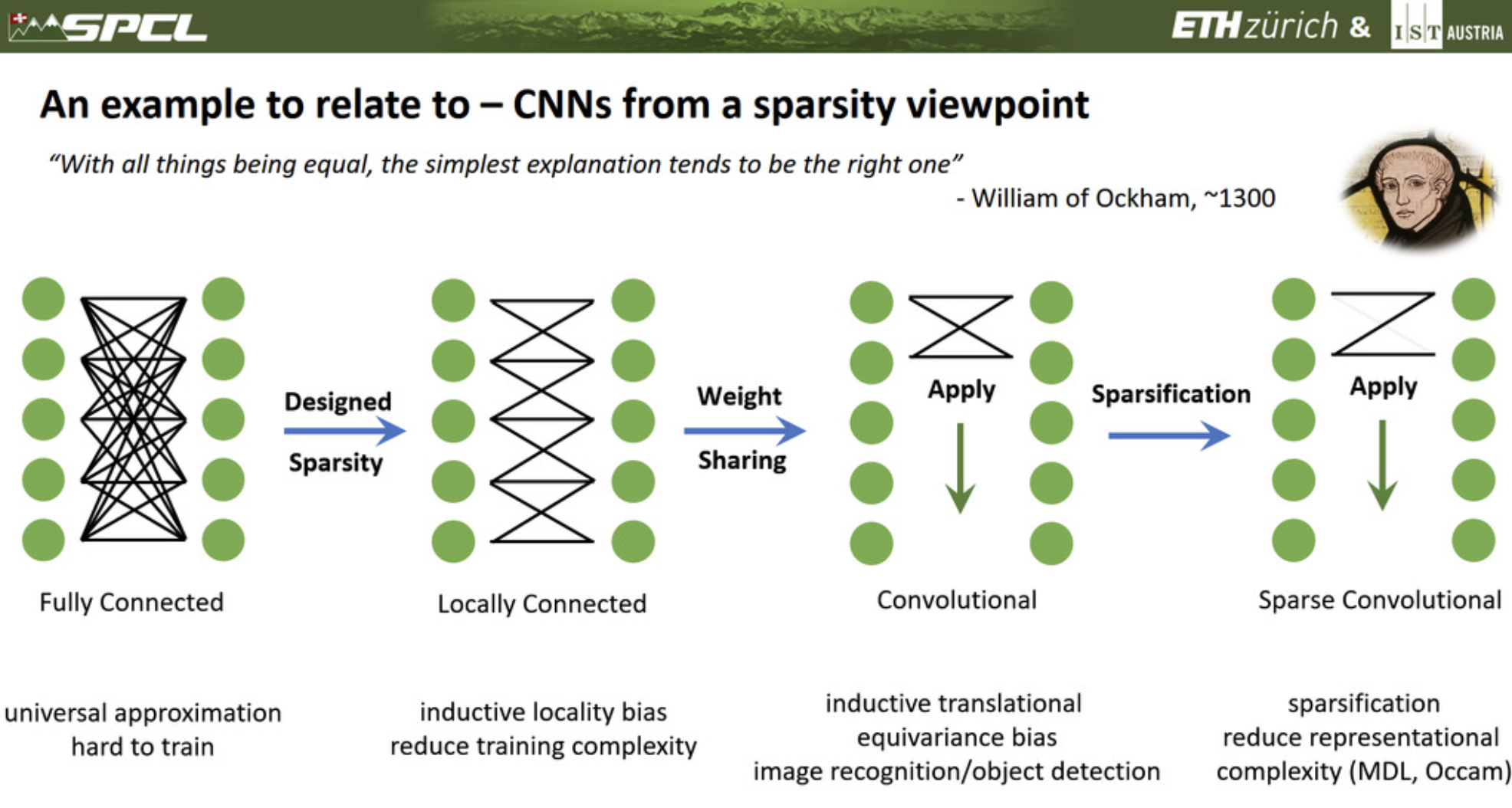
To begin with, we can actually explain the idea of convolutional neural networks (CNNs) starting from a fully connected network. If we tell the model that each neuron can only see/interact the adjacent neurons from the former layer, then it becomes a locally connected network, but it’s not a CNN yet. To achieve CNNs, we apply an additional principle, which is a locality principle. What we do is simply sharing the weight across all the inputs and outputs. From this point, we can even further sparsify the network by removing a connection, then it becomes a sparse convolutional neural network.
Wow, we can see that the connections between neurons are greatly reduced from fully connected network to sparse convolutional network. The foundamental idea behind this is that today’s networks are overparameterized. They memorize full examples and they even can learn randomly permuted labels, but do we really need this for generalization, or we just need the latent information to be represented in the network. For instance, there are even networks that 5% of the parameters are sufficient to predict the remaining 95%. Another prespective is from the Occam’s razor and the MDL principle. In theory, better generilization often results from the minimal or lower complexity stored in the model. For example, we often use dropout layer to increase the generalization, but lose the random example/feature during the training processes.
However, it’s worthy to mention that over-parameterized models are easier to train. Let’s look at the following image.
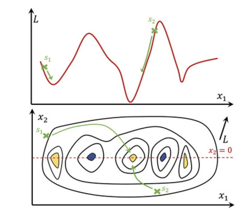
If we only have one featrue and the loss function goes into the second dimension, then it might be hard to reach to the minimum when random initialization falls on
on the top graph of the image. But if we have an additional feature
also and the loss function goes into the third dimension, then
may help
to breach to the global minimum instead of the local minimum that’s way closer to it. That’s why intuitively with more parameters it’s easier to train unto a better generilization.
Now let’s look at the following sketch of the Occam’s hill and generlization.
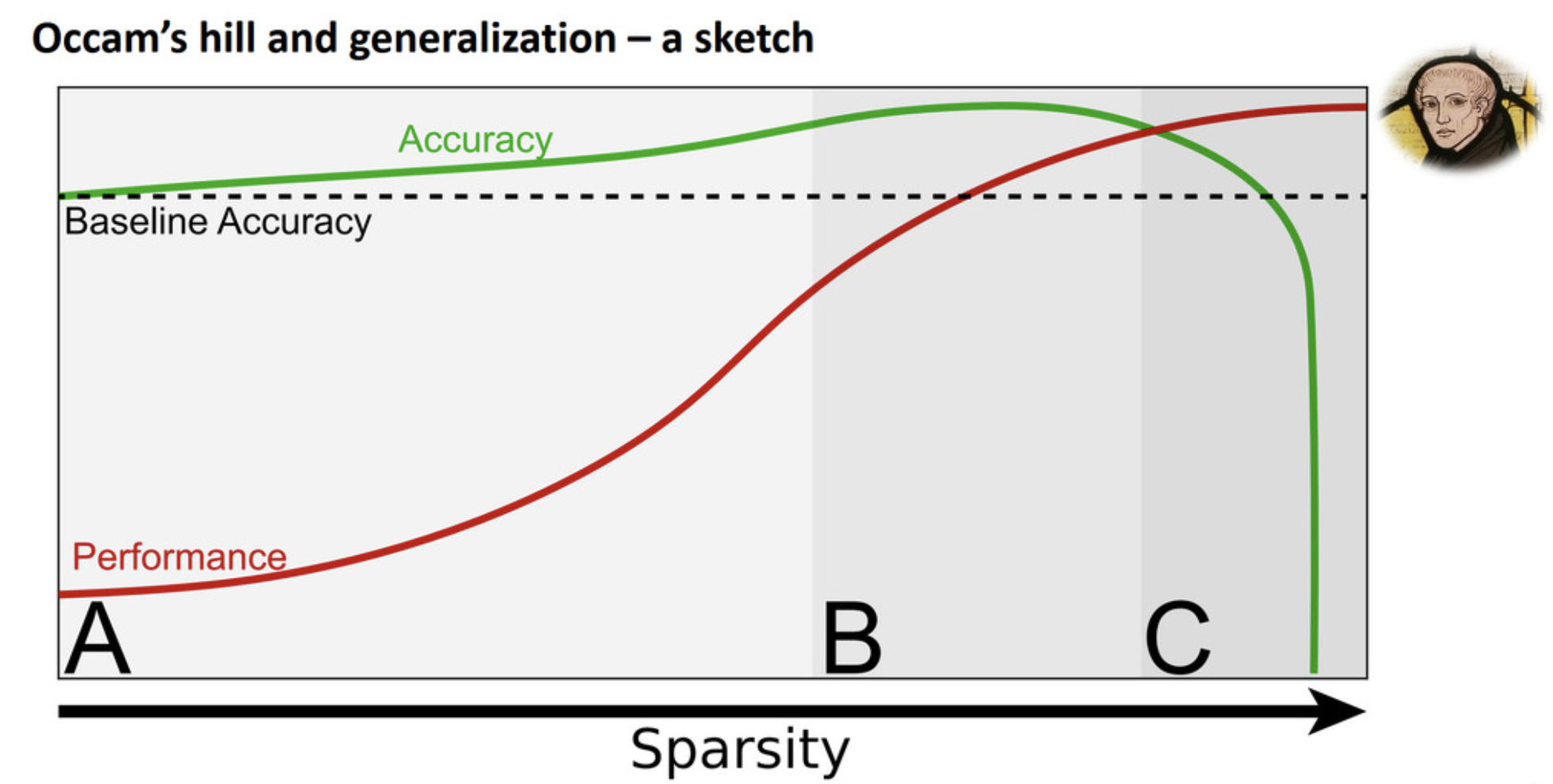
As we increase the sparsity from region A to B, we may gain some accuracy from the baseline. But when it reaches to region C, the accuracy drops dramatically. Of course we may gain some accuracy (e.g., 0.5-1%) by increasing sparisty, but that’s not the main reason that people work on sparsity. The main reason is that increasing sparsity may increase the performance of the model in terms of faster evaluation and cheaper storage.
What are the apporaches of sparsification?
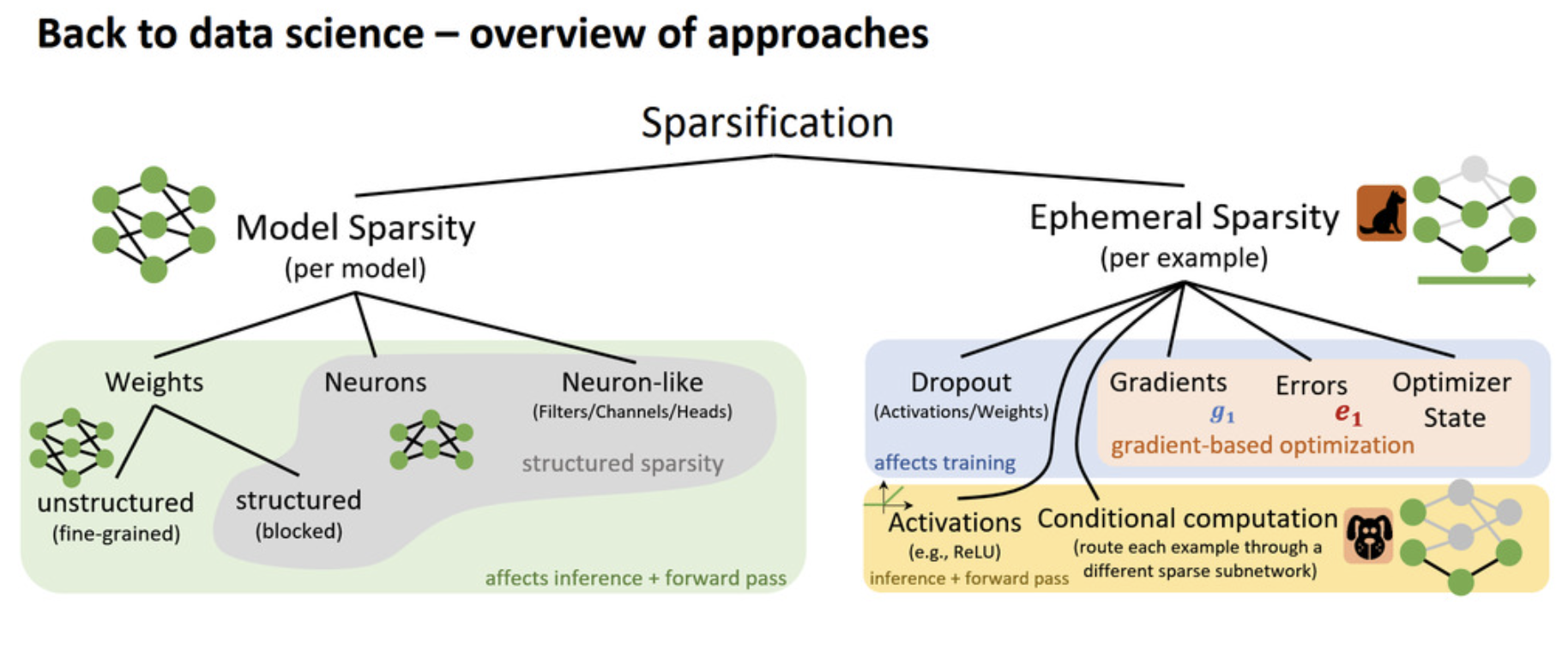
The first general apporach is model sparsification, which is somehow to thin out the model. For example, we can sparsify the weights or neurons by reducing them, and we can also sparsity neuron-like layers such as filters/channels/heads. The weight sparsification is often called unstructured sparsification because it oftens leads to a unstructued weight matrices, but it really depends on how you sparsify them. If you remove rows of weights or colomns of weights (i.e., sometimes similiar to reducing the neurons), then it can be structured sparsification. All of these above affect the inference as well as the forward pass during training.
The second general apporach is ephemeral sparsity. When model sparsity is constant, ephemeral sparsity changes on a per-example basis. Dropout (simply as its name) and activations (e.g., ReLU simply drops everything below zero) are typically ephemeral sparsity, as well as gradients, errors, optimizer states, where the-latter-three-kind-of-sparsity only applies to gradient-based optimization.
When to sparsity?
Now we know what to sparsity, but when to sparsify?
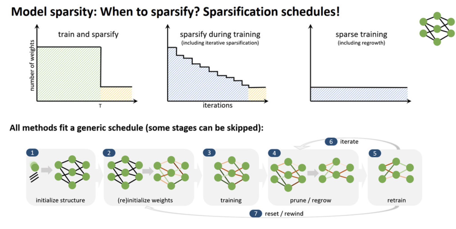
There are three very different schemes in the image above, but they can all fit a genreric schedule where some stages can be skipped. Notbly, from step 5 people may go back to step 4 to prune and regrow the network, and then retrain the model again. It’s worwhy to mention that step 7 is more of a interest of sciencetic research but not for useful pruning application.
How to select a sparsification schedule?
If we’re planning to sparsify during training, it can turn weights on/off for most efficient search, and it also enable dense-sparse-dense training schedules. This is generally beneficial to the SGD training because we can still compute the gradient of the whole paramertized model but we only consider a subset of the weights for the forward pass. Additionlly, one of the foundamental principle to understand is called the early structure adpatation. The intuition comes from neuroplasticity may reduce with age in biological brains. Some theoretical works suggest two phases of training (fast and slow). I believe maybe we also notice that a lot of time when we’re training a model, the cross-entropy loss for example will decrease faster in the early epochs, and then the second phase the loss is not so rapid with the iterations. The same idea may also apply on the sparcification schedule. Just think of in the early epochs the model structure may changes a lot but later as we finetune it, it gets more and more stable. Sparsify during training also brings the challenge of limtied computation resources such as GPU memory (especially HBM), but that brings people’s attention to fully-sparse training schedules.
Fully-sparse training schedules (like our brains)
Fully-sparse training schedules enable to train extremely high-dimensional (sparse) models. One way to do this is dynamic sparsity, which is to iteratively prune and grow during training. An example is NeST [arXiv], which is inspired biologically.
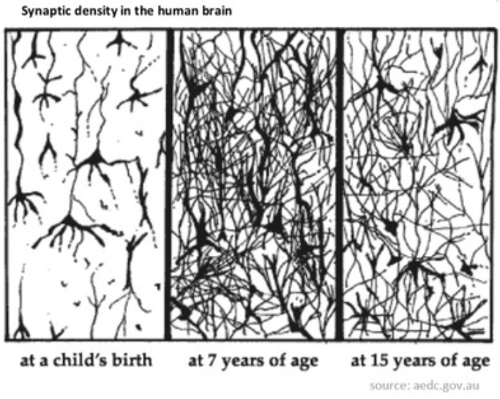
As shown in the image above:
- Random initialization (“birth brain”)
- Growth phase adds neurons and weights (“7-year-old brain”)
- Pruning phase removes neurons and weights (“15-year-old brain”)
Another scheme you can use is fully static sparsity, and a example of it is pretrained static fully-sparse schedule, which is to take advantage of early structure adaption.
For example, Single Shot Network Pruning (SNIP) [arxiv] starts with a randomly initialized network, runs a single epoch of all the data, find weights importantce meansured by sensitivity of each weight w.r.t the loss function for a single batch, remove the not-so-important weights and train the sparsified model. However, this idea falls at very high sparsity (>99%) where nearly all the weights in layers are eliminated and even disconnected.
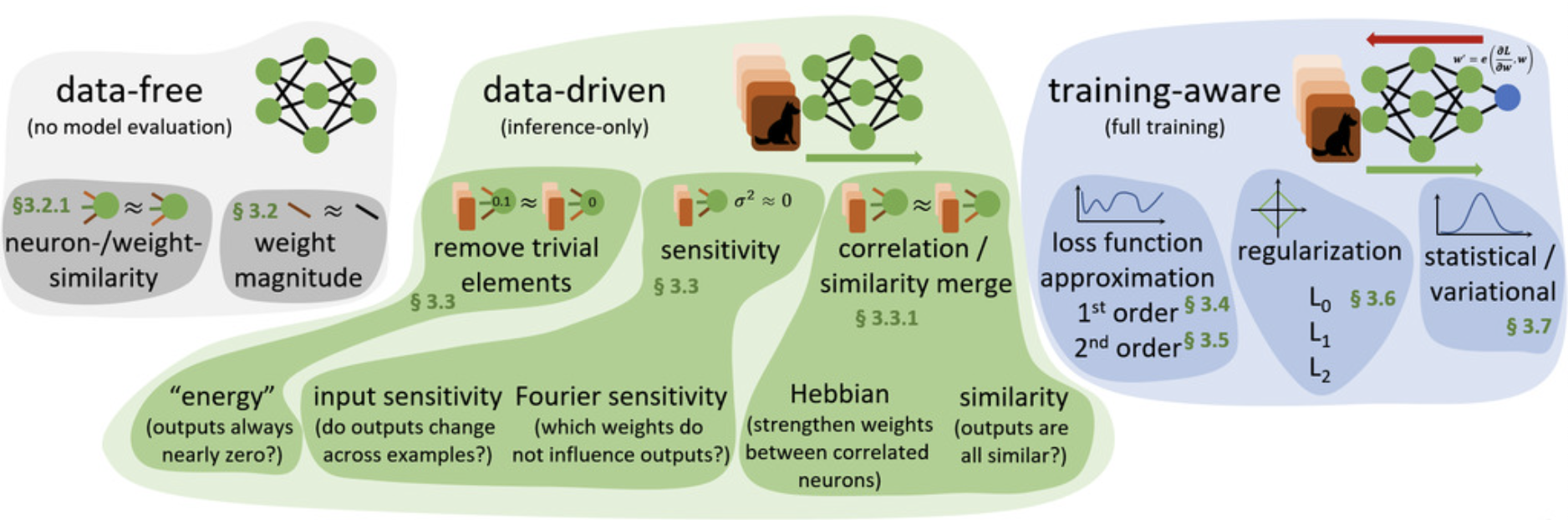
How to sparsify/remove elements?
Maybe one of the most native way is to try difference combination of sparsification. The simplest scheme is to leave out, and train
models to convergence, but it’s not efficient and even infeasible because
nowadays could be millions. So, we have to decide a selection schemes of what elements to remove by some importance metric. One of those selection methods is data-free scheme, and we only look at the model itself instead of looking at the data. For example, if I have two neurons that are essentially identical, then one of them may not be useful and hence can be removed. In addition, people can also merely look at the magnitude of the model weights. If the weights is small enough, maybe it doesn’t play an important role in this model and hence can be pruned.
On the other hand, there are also data-driven methods for selecting prunable elements. For instance, if we run a inference pass for a epoch and find a neuron with very low energy (i.e., always output a nearly zero value no matters of inputs), then maybe it can be removed because its contribution is very low. Furthermore, if a neuron doesn’t really change across many training data examples, then it may not play a differentiating role in object classification for example, so it can be removed or replaced with a constant. What’s more, what if there are neurons that are non-zero and highly correlated (i.e., always output similiar values)? Here we can either strengthen the connection with Hebbian principle or remove the larger one. These selection schemes described above can also be found in the following image.
Mathematical background
Case Studies
Ephemeral Sparsity
the future will be sparse