Group Norm, Batch Norm, Instance Norm, which is better

Gaoxiang Luo

2021-08-01

ㅤ

Batch Norm (BN)

Figure 1: Multilayer Perceptron (MLP) without BN. Credit: Lou HD

Figure 2: Multilayer Perceptron (MLP) with BN. Credit: Lou HD

PyTorch implementation of BN

1	torch.nn.BatchNorm2d(num_features, eps=1e-05, momentum=0.1, affine=True, track_running_stats=True, device=None, dtype=None)

where and are the mean and standard-deviation calculated per-dimension over the mini-batches. and are learnable parameters, where allows to adjust the standard deviation and allows to adjust the bias (i.e., shift the curve to the left or right). Most framework supports two types of evaluation mode. First, when testing, the network will use the and of the current batch statistics. Second, when inferencing (i.e., only test on a single data example), there isn’t enough data to fill a mini-batch. Hence, there are two additional parameters stored during training, which are and as a estimated mean and standard deviation of the training population (i.e., mean of all the means and standard deviations of all the batches).

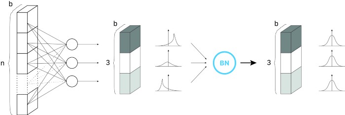
Figure 3: Example of a 3-neuron hidden layer with a batch size of b. Credit: Lou HD

At each iteration, the network computes the mean and standard deviation of the current mini-batch, and it trains and through the gradient descent.

Analysis of BN

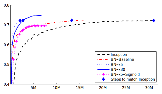
Figure 4: Batch normalization impact on training (ImageNet) Credit: [arXiv]

From the curves of the original papers, we can conclude:

BN layers lead to faster convergence and higher accuracy.
BN layers allow higher learning rate without compromising convergence.
BN layers allow sigmoid activation to reach competitive performance with ReLU activation.

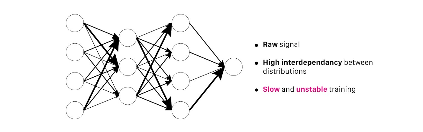
The x5 and x30 in the Figure 4 typify the multiple of learning rate from the baseline. Higher learning rate allows the optimizer to take a “brave” step and avoid local minima convergence, making it more easily converge on better solutions. In his book of deep learning, Goodfellow highly appreciated BN and it was rephased in the blog “Batch normalization in 3 levels of understanding” as the following:

Ian Goodfollow: Before BN, we thought that it was almost impossible to efficiently train deep models using sigmoid in the hidden layers. We considered several approaches to tackle training instability, such as looking for better initialization methods. Those pieces of solution were heavily heuristic, and way too fragile to be satisfactory. Batch Normalization makes those unstable networks trainable; that’s what this example shows.

For further discussion of why BN works, I found this blog is really insightful in terms of different hypothesis in recent years and why they were challenged.

However, BN has a significant shortcoming. When the batch size is very small (e.g., smaller than 8), the performance is actually degraded. It’s just like putting you and Elon Musks in the same batch for calculating the annual income. How would you feel? In addition, BN works well in image classification because you only need the critical features to classfy them. But in image stylization kind of pixel-level task, BN brings negative effect because it blurs the details of a single image. What’s more, in those dynamic networks like RNNs that require different length of input features, BN is not flexible to use.

Layer Norm (LN)

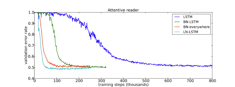
LN is quite similiar with BN. Instead of normalizing the mini-batch dimension, LN normalizes the activations along the feature dimension. Since it doesn’t depend on batch dimension, it’s able to do inference on only one data sample. In CNNs, LN doesn’t perform as good as BN or GN; however, it’s suitable in RNNs and the following is the results of applying LN on RNNs proposed by its original author.

Figure 4: Layer normalization impact on RNN. Credit: [arXiv]

PyTorch Implementation of LN

1	torch.nn.LayerNorm(normalized_shape, eps=1e-05, elementwise_affine=True, device=None, dtype=None)

where the mean and standard deviation are calculated seperately over the last certain number dimensions specified by normalized_shape. Compared to BN, LN saves lots of storage space because it doesn’t need to save the batch statistic of mean and standard deviation.

Instance Norm (IN)

IN is very similiar to LN but the difference between them is that IN normalizes across each channel in each training example (i.e., per channel per example), where LN normalizes across all features in each training example (i.e., all features per example). Unlike BN, IN layers use instance statistics computed from input data in both training and evaluation mode.

PyTorch Implementation of IN

1	torch.nn.InstanceNorm2d(num_features, eps=1e-05, momentum=0.1, affine=False, track_running_stats=False, device=None, dtype=None)

where mean and standard deviation are calculated per-dimension separately for each object in a mini-batch.

In fact, BN and IN are essentially the same thing. The different is that IN is applied to a single image while BN to a batch. But why IN could be proposed as a individual paper? If we look at BN as a task to learn the trainable parameters and , then BN can be used in domain adaption. Style transfer is a task that treats each image as a domain for domain adoption. Intuitively, IN allows to remove instance-specific contrast information from the content image in a task like image stylization. The problem that IN tries to address is that the network should be agnostic to the contrast of the original image.

Group Norm (GN)

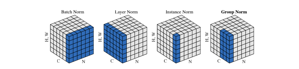
Similiar with LN, GN is also used along the feature dimension, but it divides the features into groups and normalizes each group respectively. The authors of GN were inspired by classifical computer vision techniques like SIFT and HOG descriptors, which involve group-wise normalization.

PyTorch Implementation of GN

1	torch.nn.GroupNorm(num_groups, num_channels, eps=1e-05, affine=True, device=None, dtype=None)

where input channels are splited into num_groups. The means and standard deviations are computed over each group respectively. This layer uses statistics computed from input data in both training and evaluation modes.

Re-scaling Invariance of Normalization

We know the training gets more difficult when the network gets deeper, because there exists gradient vanishing and gradient explosion issue during backpropagation. Furthermore, it also affects the model that it cannot converge or converge slowly. From the perspective of neurons’ magnitudes, if the paramters of neurons are invariant to re-scaling, then it means the huge or tiny magnitude of outputs won’t affect the training much. All sorts of normalization in a sense indeed are re-scaling invariant. It’s not why normalization is popular in deep learning community but it could be one of the blessings of normalization that deserves a discussion.

In the paper of Layer Normalization, it talks about weight vector re-scaling, data re-scaling and weight matrix re-scaling. Data re-scaling invariance typifies the activation value after normalization is the same for both and where is a constant. Weight vector re-scaling invariance means if we multiply all the incoming connections (i.e, weights) to a single neuron by a constant, then the activation value after normalization remains the same. Weight matrix re-scaling invariance stands for multiply all the connections (i.e., weights) between and layers by a constant, then the activation value after normalization is unchanged.